Analytic Functions
Arcadia Enterprise supports several analytic functions that examine overlapping groupings of data.
Analytic functions are similar to aggregate functions because both use the contents of
multiple data input rows to calculate the result. Analytic functions use flexible conditions
that are specified by the OVER(...) clause to order and group input so that
specific rows may be part of the calculation for several output values.
This article contains the following sections:
Supported Connections
Syntax for analytic functions is slightly different depending on the type of data connection used.
Supported Data Connections include the following:
The Analytic Functions field properties are not available on MariaDB, MySQL, non-Oracle SQLite, Apache Drill, and Apache Solr connections
Syntax for analytic functions is slightly different depending on the type of data connection used. Analytic functions are not available for connections to MySQL, SQLite, Drill, MS Sql Server, Teradata, Solr, KSql, and MariaDB.
- In the query execution order, analytic functions follow the
WHEREandGROUP BYclauses. Therefore, the function excludes the rows that are filtered out by these mechanisms, and they never become part of the analytic function data subset. - When using both analytic functions and ordering, the available ordering options include all fields that are on the shelves, less the fields that are on the Filters shelf. To sort a visual on the results of an analytic functions, place the field used in the analytic function onto the Tooltips shelf.
- Use Enter or Edit Expression option for running analytic functions that are not automated within Arcadia Enterprise.
The rest of this topic covers the basic steps of accessing the analytic functions, and the basic visual set-up that we use in subsequent topics, to demonstrate each analytic function.
Basic Steps
To use analytic functions, follow these steps.
Open the visual where you want to specify an analytic function, in Edit mode.
In this section, we use a line visual defined in the Basic Visual for Aggregates example.
On a measurement shelf of a visual, click the field you plan to modify to open the Field Properties menu.
In our examples, we use the population field on the X Axis shelf.
-
In the Field Properties menu, click to expand the Analytic Functions menu.
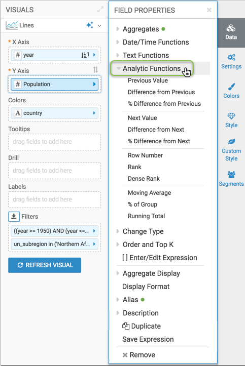
Select one of the following analytic functions, directly supported by Arcadia Enterprise:
In addition to these, you may use the expression builder to specify other analytic functions. See Enter or Edit Expression.
Basic Visual for Aggregates
Here, we create a basic line visual on the World Life Expectancy dataset,
through an Arcadia data connection. In subsequent topics, we use this visual to demonstrate
how the various analytic functions for aggregates work.
- Open a new visual.
- In the Visuals menu, select the Lines visual type.
Populate the shelves of the visual from the fields listed in the Data menu:
- X Axis
Add the field
year. Order it in ascending order. - Y Axis
Add the field
population. - Colors
Add the filed
country. Order it in ascending order. - Filters
Add the field
year, and set it to the interval of 1950 through 2010.Add the field
un_subregion, and set it to Northern Africa.
- X Axis
Click Refresh Visual to see the new line visual.
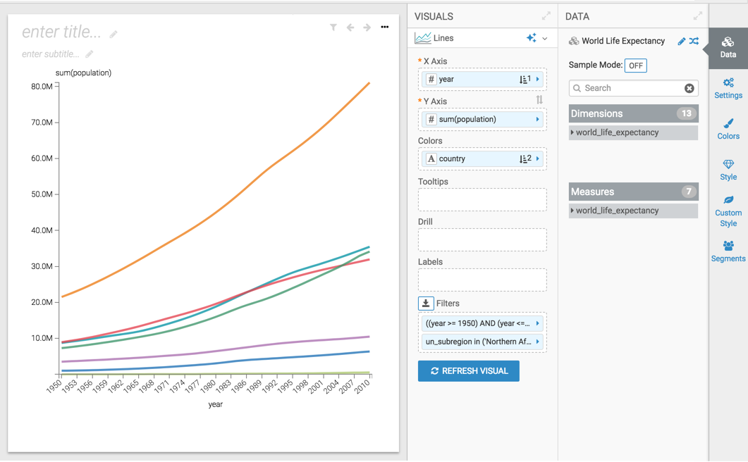
- Name the visual Basic Lines.
- Click Save.
Basic Visual for Single Values
Here, we create a basic table visual on the World Life Expectancy dataset,
through an Arcadia data connection. In subsequent topics, we use this visual to demonstrate
how the various analytic functions for single values work.
- Open a new visual.
- In the Visuals menu, select the Table visual type.
Populate the shelves of the visual from the fields listed in the Data menu:
- Dimensions
Add the fields
country,life_expectancy,gdp_per_capita, andpopulation. - Filters
Add the field
year, and select the value 2010.Add the field
un_subregion, and set it to Africa.
- Dimensions
- Specify descending order on
life_expectancy. [Optional] In the Enter/Edit Expression editor, change the
gdp_per_capitacalculation on the shelf, and rename it:[gdp_per_capita]*[population] as 'GDP'- [Optional] Change the Display Format options for the fields on the shelves to remove extra decimals, specify currency, and so on.
- [Optional] Change the Alias for the fields on the
shelves.
Click Refresh Visual to update the table visual.
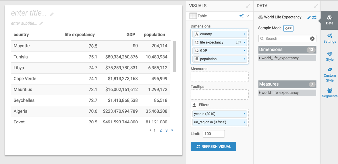
- Name the visual Basic Table.
- Click Save.